Differentiable Engineering

Executive summary

• By including differentiable, parametric models in engineering processes, engineering software can better interoperate between human and artificial designers.
• Existing CAD, CAM, and CAE tools can speak this language by adding differential interoperability to their APIs.
• We provide a visual introduction to differential engineering using a cantilevered beam.
• By examining the derivative of a rotation, we briefly unlock some deep math beauty and an application of Unit Gradient Fields (UGFs).
• Differentiable engineering scales to product-level systems engineering.

✏️ Math advisory: this post assumes you’re okay with derivatives, the chain rule from basic calculus, and a little vector math. We will introduce intuitive visual tools to illustrate such concepts in design engineering. While I feel compelled to show the work, you can probably skim and glean the concepts from the illustrations.

👥 Lots of credit: These ideas came from discussions with many people, including:

• Sandilya (Sandy) Kambampati, Intact Solutions
• Luke Church, Gradient Control Laboratories
• Trevor Laughlin, nTop
• Jon Hiller, PTC
• Peter Harman, Infinitive

Introduction

Today, we practice three paradigms of computer-aided design (“CAD”), manufacturing (“CAM”), and engineering (“CAE”):

• One-off design, where the focus is producing individual parts or products;
• Parametric generative design, where the result is recipe to produce variants of similar parts or products; and
• Computational generative design, where the final geometry is guided by simulation, often iteratively and with spatially-varying parameters.

As each of these generations has built on earlier technology, the emerging generation of engineering software powered by artificial intelligence and machine learning algorithms (“AI/ML”) is being trained on existing empirical, simulated, and textbook knowledge. However, while this new generation of tools promises ease-of-use, more accurate results, and orders of magnitude faster performance, it does not yet offer a meaningful shift in interaction paradigm. As these new tools become increasingly sophisticated, will new interaction paradigms emerge? Will we realize the sci-fi vision of product-level generative co-designers?

Let’s examine how AI and ML can blend with today’s optimization tech to expand engineers’ navigable design space. As generative design scales to the subsystem and product level, we’ll demonstrate how to delegate tasks to AI and ML without the meaning becoming hidden in a nonintuitive latent spaces, as with LLMs and generative art. We’ll focus on the role of a designer, human or automated, expressed in the language of optimization and machine learning: a differentiable approach to design engineering.

Abstracting the design engineer

Let’s propose a model for a design engineer, human or automated, which we’ll call “Mechanical Design Automation (MDA)”:

\(\newcommand{\Shape}{\Omega}\) \(\newcommand{\parameters}{\boldsymbol{\Theta}}\) \(\newcommand{\fitness}{\boldsymbol{F}}\) \(\newcommand{\CAD}{\text{CAD}}\) \(\newcommand{\CAE}{\text{CAE}}\) \(\newcommand{\MDA}{\text{MDA}}\)

There are three main roles in an engineering process:

• Model creation tools, like CAD and CAM systems, generate output like parts, assemblies, and manufacturing deliverables. We can model CAD as a function from parameters \(\parameters\) to designs or “shapes” \(\Shape\), \(\CAD\!: \parameters \mapsto \Shape\). We’ll focus on simple dimensional and angular parameters as in parametric CAD, but other parameter types include the feature recipe, explicit positions of mesh vertices, density values on a voxel model, material selection, etc.
• Engineering (CAE) tools measure various fitnesses \(\fitness\) of CAD designs, such as mass properties, testing mechanical and other physical properties, cost, environmental impact, and aesthetics. We can model engineering software as \(\CAE\!: \Shape \mapsto \fitness\).
• Finally, there is a designer interested in producing optimal designs by tuning the parameters to optimize fitness. \(\MDA\!: \parameters \mapsto \Shape \mapsto \fitness = \parameters \mapsto \fitness\). The design Jacobian, described below, informs the designer how to update parameters to improve fitness.

✏️ Math tip: the notation \(f: x \mapsto y\) defines the function \(y = f(x)\) and can be read as “maps to.”

The designer’s shape paradox

This system suggests that a designer cares not about the shape of their design, only its fitness. Paradoxically, most design engineers focus their work on drawing and documenting shapes! If industrial design and assembly context are taken as constraints, perhaps nonintuitive, topology optimized results are closer to home than we thought.

On the other hand, this model shows that a designer is most interested in navigating an available set of design parameters explore a large design space of shapes to achieve a fitness goal. Somehow, the designer needs to use a set of fitnesses to update the set of parameters. And we only have one shape \(\Shape\) for every vector of input parameters \(\parameters\) and vector of fitnesses \(\fitness\).

What is the map from fitnesses to parameters? It’s the inverse of MDA, the origin story for the term “inverse engineering.” In many cases, we might optimize a design by minimizing a scalar “loss function.” Various optimization techniques such topology optimization and multi-disciplinary optimization (MDO) are examples of this setup.

How should a design engineer optimize a set of parameters to achieve the fitnesses that maximally satisfy all stakeholders, while also being theoretically unconcerned about the output shape? Given any shape and fitnesses, the designer must tweaks the design until it’s optimal. In such a world, it might be helpful to know in what direction and how far to adjust a parameter for the intended result. The tools of calculus provide such an estimate.

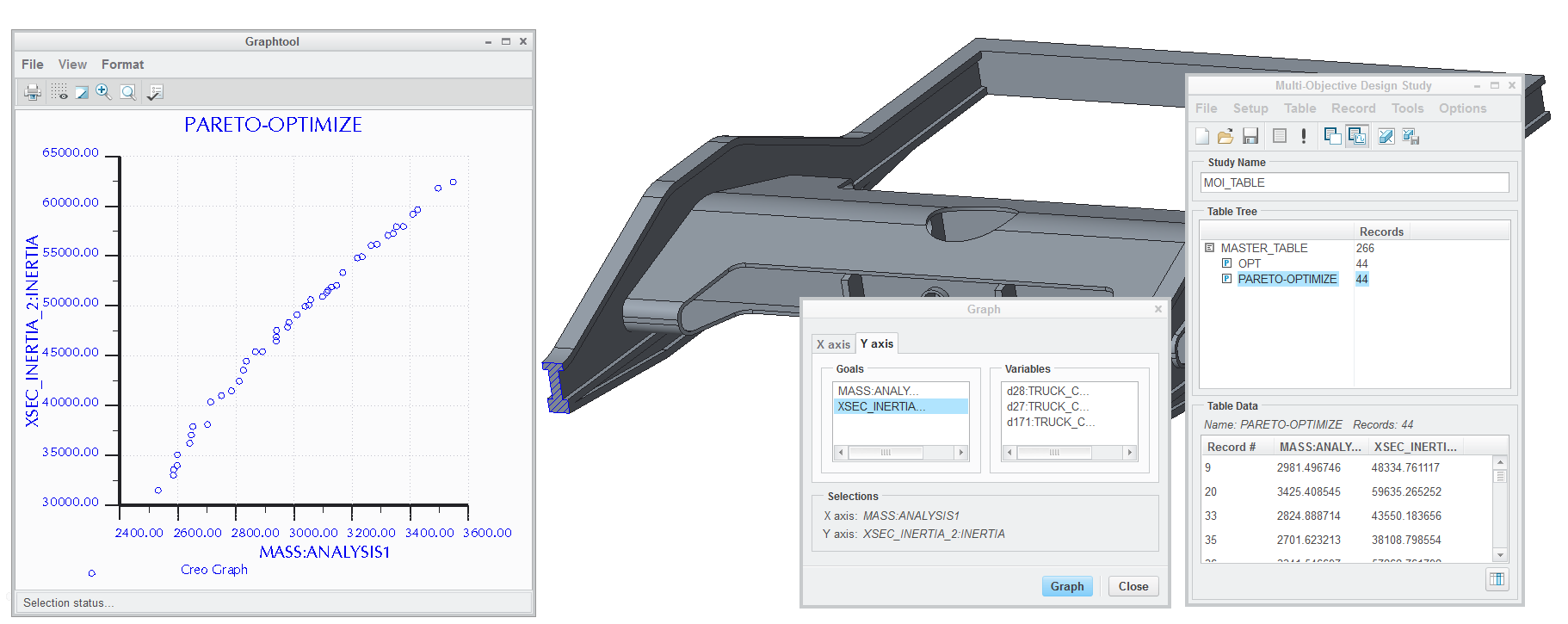
Behavioral modeling in Creo aka “Pro/E”, courtesy of PTC. The plot shows a Pareto front of the trade-offs between two different fitness components while varying spatially constant parameters. Differentiable engineering can efficiently find and smooth such curves in a similar way to how CAD systems trace precise silhouette curves of curved surfaces in hidden-line views. (Silhouette curves are Pareto fronts, trading off the surface’s UV coordinates for coordinates on the projection target!)

When I was just out of college as an PTC application engineer selling Pro/E, I used to demo parametrically optimizing a part through FEA. The first thing the solver would do is make a small change to the parameters to compute a slope to find the optimal value and iterate until it was close enough. The terms “gradient descent” and “Newton’s method” describe this process. In those days, it would take some time to regenerate the CAD part for each parameter set, so you had to do some story telling while it was computing that slope. In today’s state of the art, like nTop field optimization, we iterate over a similar loop, but with spatially varying fields, providing generalized shape and topology optimization for open-ended problems.

Field optimization in nTop, animated by Brad Rothenberg. One spatially varying parameter, wall thickness, minimizes the deflection of a cantilever (fixed on the left, loaded on the right).

Enter the derivative

It sure would have been nice if Pro/E knew that slope right away, freeing the optimizer from regenerating and simulating another variant just to estimate a derivative. As popularized by recent trends in machine learning, three forms of automatic differentiation enable us to more efficiently compute such parametric sensitivities:

• Symbolic differentiation: If we have a mathematical expression, we can differentiate it one variable at a time to produce a new function for each derivative of interest.
• Forward mode automatic differentiation: Equivalent to the fascinating dual numbers, we maintain and update each parameter’s derivative with its value with every operation on its value. It can be straightforward to convert conventional code to forward mode using types.
• Reverse mode automatic differentiation: When computing, we build a structure that can be used to compute derivatives later, which is efficient when you have many inputs and only a few outputs. When differentiating though FEA and CFD simulations, a technique called the adjoint method makes reverse mode computationally efficient.

👥 For more nuance about automatic differentiation in optimization algorithms, see Nick McCleery’s thorough post on differentiable programming in engineering.

We now arrive at the heart of differentiable engineering, the chain rule through a shape:

✏️ Math tip: read the partial derivative notation “\(\partial x\)” as the same as “\(dx\)” assuming all partials are independent, but be aware that there are more of them. If \(\p = (x, y)\), we express a vector of those partials as the gradient \(\grad f(\p) = \pdv{f}{\p} = \left(\pdv{f}{x}, \pdv{f}{y}\right)\), notation we reserve for spatial derivatives.

Speaking in the language of differentials (and linear algebra):

• CAD systems are concerned with shapes’ parametric sensitivities \(\pdv{\Shape}{\parameters}\) (a row vector);
• CAE systems determine shapes’ functional sensitivities \(\pdv{\fitness}{\Shape}\) (a column vector); and
• MDA becomes the (outer) product of those two vectors, a matrix of derivatives that captures how each parameter contributes to each fitness. Such a matrix of partial derivatives is called a “Jacobian”, so it seems appropriate to call \(\pdv{\fitness}{\Shape} \pdv{\Shape}{\parameters}\) the design Jacobian.

All design engineers, human or automated, serve to optimize the fitness of stakeholder deliverables via design Jacobians.

What \(\pdv{\fitness}{\parameters} = \pdv{\fitness}{\Shape} \pdv{\Shape}{\parameters}\) shows is that CAD tools can pass along differentials to CAE tools to compute design Jacobians. It shows that CAD and CAE vendors can work together to provide differentiable answers to engineers and optimization systems. Our industry has done it before: the Functional Mock-up Interface standardizes analogous interoperability over time derivatives to model one-dimensional, dynamic systems.

While the parameters may or may not vary spatially, we tend to evaluate the fitness of the entire shape, often by integrating over space. For example, the volume and surface area fitnesses are integrals over a shape’s domain and its boundary, respectively. Maximum, minimum, or average values like center of gravity may also roll-up fitness to a constant value. Note that the parametric derivatives become tallied up in such spatial integrations or consolidations. Field optimization implies that some spatially varying parameters do not get consolidated.

Visualizing derivatives as fields

Let’s work through a simple engineering example: a cantilevered beam. We will represent it as an exact SDF for comparison with Mercury and IQ’s haikus, which are optimized for the GPU but complicate taking the derivative.

A rectangle and its derivatives

For our shape \(\Shape\), we’ll use a rectangle \(\shape{R}(\p; \point{s}_½)\) centered on the origin with size \(\point{s} = (w, h)\). Due to symmetry, we’ll parameterize via the half-size vector \(\point{s}_½ = \left(\frac{w}{2}, \frac{h}{2}\right)\), our parameter set (\(\parameters\) above). Given position \(\p\), let’s define:

where \(\abs{\cdot}\) is the absolute value of the components, which provides us with positive local coordinates centered on a corner of the rectangle. It’s as if we folded the rectangle in half twice and can now just work on the one corner. Then, given components of \(\p_c = (\p_{cx}, \p_{cy})\) and Euclidean norm (aka vector magnitude) \(\norm{\cdot}\), case-wise, we handle the regions closest to the vertex and then each side:

Let’s get a feel for rectangle field and its partial derivatives (click to sample the field):

What does it mean that the derivatives have value off of the boundary of the shape? Isn’t there only one shape? Yes, but under any offset of a shape by a constant, \(\Shape - \lambda\), the derivative of the offset \(\lambda\) vanishes. This magic X-ray vision (aka “first order approximation”) of derivative fields results in such constant values along streamlines of the gradient, creating a field radiated into and out of the shape from the boundary.

Deriving the derivatives

The case-wise construction simplifies taking derivatives, as the same cases apply. Here is our spatial gradient, which always points to the boundary:

and our derivatives with respect to the half-size vector components:

Why the negative values? As the rectangle becomes bigger, the field values at locations on either side of it become smaller.

What if we want the derivatives with respect to \(w\) and \(h\)? \(\pdv{\point{s}_½x}{w}\) and \(\pdv{\point{s}_½y}{h}\) are both \(\frac{1}{2}\), so \(\pdv{\shape{R}}{\point{s}} = \frac{1}{2} \pdv{\shape{R}}{\point{s}_½}\) .

Chaining in the fitness functions

Let’s introduce some fitness properties (\(\fitness\)) for our rectangle \(\shape{R}\), which, despite its symmetry, could be a cantilevered beam adding depth \(d\). We’ll fix one side and put a downward load \(f\) on the other. We can then write down our textbook deflection formula for volume \(V\), sectional inertia \(I\), and deflection \(\delta\) given constant elastic modulus \(E\):

Which are clear functions of the basic dimensions of \(\shape{R}\). We don’t need to pull out the chain rule through a shape, as that work is already baked into these formulae from the integrals in their construction. Observe that the volume calculation for our cuboid beam is equivalent to an approximate Riemann integral with one big element. We can work with any kind of geometry across which we can integrate, the trick used by meshless approaches to simulate physics on geometry unsuitable for finite element meshing. Intact Solutions focuses on this kind of approach to simulation, and toolkits like FEniCS provide a differentiable physics when meshing is convenient.

Here, we can just analytically differentiate with respect to \(point{s}\):

These values, the rows of our design Jacobian \(\pdv{\fitness}{\parameters}\), are constant with respect to space.

Shape, topology, and field optimization

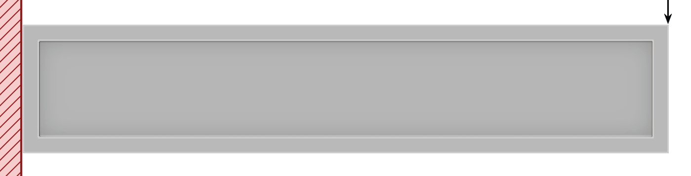
Modern optimization tools add more parameters to the model, for example this parameterized cantilever from Sandy at Intact, optimized using derivatives with respect to paameters at each arrow:

Other kinds of shape optimization might use the positions of mesh vertices or subdivision surface control points. Topology optimization extends this concept using voxel-based parameters for density or implicit boundary values.

Transforming our shape

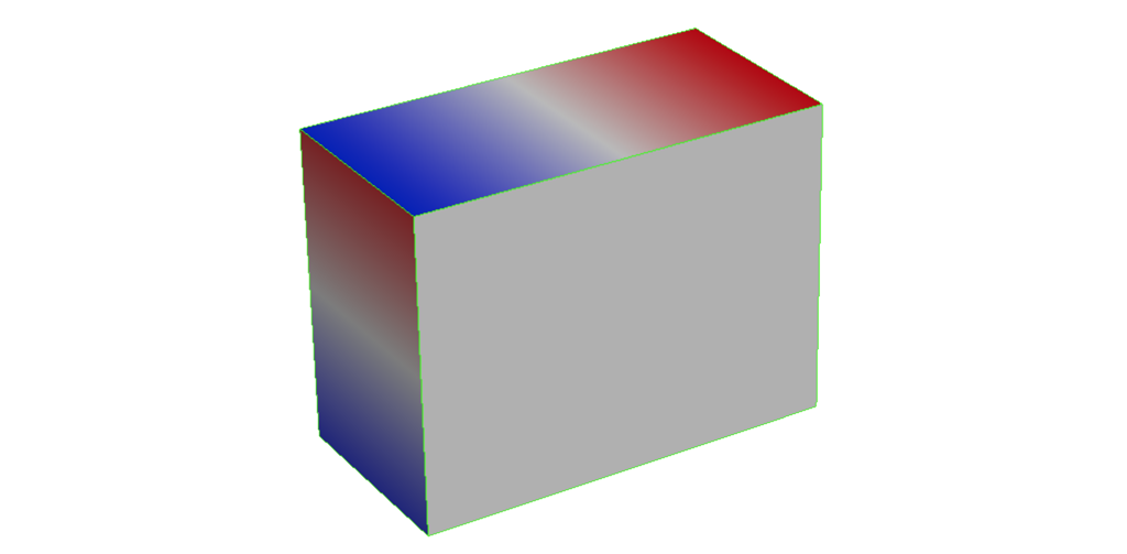
Let’s take a look at the derivative of rotating a shape, noting that a translation leaves the derivative unchanged. As our rectangle rotates about its center, we can measure how much each increment adds material to or removes material from each face. Another way to think about this rotational derivative is how much each surface element would be facing wind or in the lee of the wind while it turns. In regions where the material is being added, the derivative is negative, the same sign conventions as when resizing the rectangle.

Let’s start by illustrating the rotational derivative on explicit geometry. Using differentiable boundary models, it’s possible to compute such derivatives directly on the surface. For example, here is the rotational derivative through the center of the box visualized on the faces using Engineering Sketch Pad.

The derivative of a rotation

As a casual mathematician, it’s rare to get a window into the inner workings of math. The rotational derivative our rectangle provides such an opportunity. Consider rotating our rectangle \(\shape{R}(\p; \point{s}_½)\) through its center by angle \(\alpha\) by remapping via the transformation \(T(\alpha)\!: \p \mapsto \p'\), where:

Differentiating with respect to \(\alpha\):

Therefore, taking the derivative of a rotation is the same thing as adding a quarter turn to the rotation, evidence of some deeper math. In complex analysis, we learn this operation as multiplying by \(i\). In differential forms, we have the complex structure \(J\) that lets us perform rotations on surfaces. Geometric generalizes the notation to rotors. All of these concepts square to \(-1\).

Before we perform its derivation, let’s take a look at \(\pdv{\shape{R}}{\alpha}\) with fields rotated through the center of the image. The animation shows the complex structure of the derivative of a rotation by superimposing it with the original field. We illustrate the rotation by creating a family of (“pencil”) by performing rotational interpolation on \(\shape{R}\) and \(\pdv{\shape{R}}{\alpha}\):

while animating \(\phi\):

How to interpret the animation? It’s similar to the rotating box, but we are holding the shape fixed and rotating space around it, which seems to me to be the nature of the complex structure induced by a rotation. Observe that the rotating space passes through the boundary almost as if we were observing the wind on the rotating box, but from the reference frame of our rectangle.

The rotational derivative of a field

Let’s take the derivative of \(\shape{R}(\p')\) with respect to \(\alpha\), \(\pdv{\shape{R}}{\alpha}\). We start with the rotated scalar field \(\shape{R}(\p')\), where \(\p' = T(\alpha)\,\p\) is the rotated position vector:

Using the chain rule on the second term, we have:

Substituting into the earlier expression and defining our quarter-turned \(\p\) as \(\p_i \equiv T\!\left(\frac{\pi}{2}\right) \p\):

✏️ Math tip: \(\nabla_{\p'}\shape{R}\) shows the gradient \(\pdv{\shape{R}}{\p'}\) that in the spatially transformed basis \({\p'}\).

In 2D, \(T\!\left(\frac{\pi}{2}\right)\!: (x, y) \mapsto (-y, x)\), the same operation as multiplying \(x + iy\) by \(i\).

Connection to Unit Gradient Fields (UGFs)

If we are interested in \(\pdv{\shape{R}}{\alpha}\) for an unrotated object, we can set \(\alpha = 0\), so \(T(\alpha)\) becomes the identity:

As our rotation \(T\) is a rigid motion, if \(\nabla_{\p}\shape{R}\) has the property that its gradient (everywhere defined) is unit magnitude, so does the transformed \(\nabla_{\p'}\shape{R}\). Therefore, the property that avoids stretching in the rotational derivative is the property of having unit gradient magnitude, the defining property of UGFs (and of which SDFs are subset). (If you dare try an implicit shape specified with a non-Euclidean metric instead of a UGF, open the Shadertoy and uncomment line 91.)

Differential systems engineering

Once we have CAD and CAE systems wired to compute design Jacobians via \(\pdv{\fitness}{\parameters} = \pdv{\fitness}{\Shape} \pdv{\Shape}{\parameters}\), we can connect them into PLM frameworks and consider systems models of process- and product-scale generative design. For example, consider the problem of finding the optimal orientation to place a part in advanced manufacturing, where perhaps we want to minimize material consumption use while also minimizing deflection:

Given our placed CAD part \(\Shape(w, h, \alpha, \ldots)\), our supports \(\Psi(\Shape, \ldots)\), and fitnesses such as volume of \(\Psi\) and max deflection \(\delta\), then:

When we derive one CAD model from another, as common in tooling like molding and casting, we can pass the differentials along via the chain rule. This process of modifying part geometry to improve manufacturing processes we call “design for manufacturing.” How far can go to model and trace such sensitivities, unlocking causality typically obscured by disjointed PLM processes?

What about derived parts through assembly and product structures? How would such sensitivities propagate? Multiple parts could contribute to parent CAD assemblies. Consider, for example, parts \(\Shape_1(\parameters_1)\) and \(\Shape_2(\parameters_2)\) assembled into Assembly \(\Shape_A\) via assembly placement parameters \(\parameters_A\) including separation distance \(d\):

Then:

and given analogously named fitnesses:

This structure mirrors the V model of systems engineering, where a design process commences with high level fitness requirements and becomes subdivided into subsystems, subassemblies, and finally individual components for detailed design at the bottom of the V. One the way back up, integration and validation processes assure that the component-level fitnesses assemble into product-level fitnesses. These differentiable engineering pipelines appear to fit naturally into such PLM and product development methodologies.

As artificial intelligence becomes increasingly present in our engineering tools processes, differentiable engineering’s inherent compatibility with the V model may expedite integrating human engineers with artificial design aides to maximize product-scale product fitness. By modeling not only product content but how it evolves though it’s differentials, AI and ML may transform generative CAD and CAE into a new paradigm of mechanical design automation. While we are still imagining what form these new tools might take, it seems clear that they will connect via differentiable engineering.

Background and credits

With the launch of interactivity in nTop 3.0 three years ago, George Allen and I shared some research around “CodeReps”, which showed how we could export nTop data as pure code. Sandy from Intact not only performed simulations on these code reps, he also observed that we could take parametric derivatives of it for the purpose of optimization, should CodeReps become pervasive. Trevor from nTop also saw potential of geometry to be a parametric black box for optimization routines. Matt Keeter showed how to use such derivatives for parametric editing in libfive studio when explicitly declared, and Luke Church prototyped a 2D implicit modeler that provided UX on-the-fly with respect to local parametric sensitivities.

Around that time I started to notice the use of differentiable simulation pipelines, both in open source packages like FEniCS and research using the adjoint method. As Sandy started to show differential results via adjoints, my friends at Atomic Industries started building a fully differentiable modeling-through-multiphysics pipeline to train their AI to optimize mold design. About a year ago, Jon Hiller and I started regular conversations about the future of implicit modeling and generative design, and we became engaged in the challenge of federating separate CAD, CAM, and CAE tools through differentiable interfaces throughout PLM. Would it be possible to design such APIs to support the different differentiation techniques, such as forward, reverse, and symbolic approaches in a manner that could scale to product definitions? The 3D printed support challenge became our main working example.

In researching existing differentiable engineering tools, Peter Harman explained the strengths and weaknesses of FMI’s approach to parametric, differentiable interop and shared his experiences with symbolic differentiation in Modelica. Eventually, I test drove Engineering Sketch Pad and met Afshawn from Open Orion, who is making explicit differential tech usable for design engineers.

2024 appears to be a great year for differential engineering. In addition to the emerging tech above, nTop’s new kernel is built for derivatives, providing industrial strength support for automation and interop. Gradient Control Laboratories’ meta-kernel generates forward-mode AD while generating other useful manipulations like symbolic derivatives and UGF transformations. I expect both technologies to be used as black boxes to realize the first generation of differential interoperability.

Are you interested in using differentiable engineering across engineering tool chains? Please get in touch!

Dedication

As I was finishing this post, it crossed the wire that Ken Versprille, the father of NURBSs and industry friend, has passed. I would have enjoyed hearing his thoughts on this material.